

Homeomorphism: Difference between revisions
| Line 45: | Line 45: | ||
== Examples == | == Examples == | ||
=== Open interval | === Open interval === | ||
The [[open interval]] <math>(0,1)</math> is homeomorphic to <math>\mathbb{R}</math>. | The [[open interval]] <math>(0,1)</math> is homeomorphic to <math>\mathbb{R}</math>. | ||
{{Proof|proof=The map <math>f:(0,1)\to \mathbb{R}</math> defined by | {{Proof|proof=The map <math>f:(0,1)\to \mathbb{R}</math> defined by | ||
| Line 53: | Line 53: | ||
is continuous. Thus <math>f</math> is a homeomorphism.}} | is continuous. Thus <math>f</math> is a homeomorphism.}} | ||
=== | === Stereographic projection === | ||
The [[Euclidean plane]] <math>\mathbb{R}^2</math> is homeomorphic to the [[2-sphere]] minus one point, denoted <math>S^2 \setminus \{N\}</math> where <math>N=(0,0,1)</math> is the [[north pole]]. | The [[Euclidean plane]] <math>\mathbb{R}^2</math> is homeomorphic to the [[2-sphere]] minus one point, denoted <math>S^2 \setminus \{N\}</math> where <math>N=(0,0,1)</math> is the [[north pole]]. | ||
| Line 144: | Line 144: | ||
}} | }} | ||
=== | === Quotient space === | ||
The unit interval <math>[0,1]</math> with the endpoints identified (the quotient space <math>[0,1]/\sim</math> where <math>0\sim 1</math>) is homeomorphic to the circle <math>S^1</math>. | The unit interval <math>[0,1]</math> with the endpoints identified (the quotient space <math>[0,1]/\sim</math> where <math>0\sim 1</math>) is homeomorphic to the circle <math>S^1</math>. | ||
{{Proof|proof=Define the map <math>f:[0,1] \to S^1</math> by <math display="block">f(t)=(\cos(2\pi t), \sin(2\pi t))</math> | {{Proof|proof=Define the map <math>f:[0,1] \to S^1</math> by <math display="block">f(t)=(\cos(2\pi t), \sin(2\pi t)).</math> This map is continuous and [[Surjection|surjective]], and satisfies <math>f(0)=f(1)=(1,0)</math>. | ||
Consider the equivalence relation <math>\sim</math>, and let <math>q:[0,1]\to [0,1]/\sim</math> be the [[quotient map]]. By the [[universal property]] of the quotient map, there exists a unique continuous map <math>\tilde{f}: [0,1]/\sim \to S^1</math> such that <math>\tilde{f} \circ q = f</math>; that is, the following diagram commutes. | Consider the equivalence relation <math>\sim</math>, and let <math>q:[0,1]\to [0,1]/\sim</math> be the [[quotient map]]. By the [[universal property]] of the quotient map, there exists a unique continuous map <math>\tilde{f}: [0,1]/\sim \to S^1</math> such that <math>\tilde{f} \circ q = f</math>; that is, the following diagram commutes. | ||
| Line 245: | Line 245: | ||
== Counterexamples == | == Counterexamples == | ||
<math>\mathbb{R}</math> is '''not''' homeomorphic to <math>\mathbb{R}^2</math>. | <math>\mathbb{R}</math> is '''not''' homeomorphic to <math>\mathbb{R}^2</math>. | ||
| Line 307: | Line 305: | ||
</div> | </div> | ||
Hence, no such homeomorphism exists; therefore <math>\mathbb{R}</math> is not homeomorphic to <math>\mathbb{R}^2</math>}} | Hence, no such homeomorphism exists; therefore <math>\mathbb{R}</math> is not homeomorphic to <math>\mathbb{R}^2</math>}}The map from the interval <math>[0,1)</math> to the 1-sphere <math>S^1</math>, | ||
The map from the interval <math>[0,1)</math> to the 1-sphere <math>S^1</math>, | |||
<math display="block">\phi: [0,1)\to S^1,\quad x\mapsto e^{2\pi ix}</math> | <math display="block">\phi: [0,1)\to S^1,\quad x\mapsto e^{2\pi ix}</math> | ||
is continuous and bijective, but not a homeomorphism. | is continuous and bijective, but not a homeomorphism. | ||
Revision as of 15:42, 1 April 2026

A homeomorphism is a special type of function between two topological spaces, that establishes that the two spaces are fundamentally the same from a topological perspective. Specifically, it is a continuous bijective function whose inverse function is also continuous. Homeomorphisms are the isomorphisms in the category of topological spaces  , which preserves all topological properties of a topological space. If such a function exists between two spaces, they are said to be homeomorphic.
Intuitively, two spaces are homeomorphic if one can be continuously deformed into the other by stretching, bending, and twisting, without cutting, tearing, or gluing. A typical intuitive example is that a mug with a handle is homeomorphic to a donut. This concept is distinct from homotopy equivalence, which allows deformations that involve collapsing. For instance, a solid ball can be continuously shrunk to a point by a homotopy, but such a deformation is not a homeomorphism because it is not bijective and the inverse would not be continuous.
Definitions
A function  between topological spaces
  and
and  is called a homeomorphism, if:
- is continuous,
- is bijective,
 is continuous.
Two topological spaces and are called homeomorphic if there exists a homeomorphism between them, denoted  .
.
Equivalent Definitions
A homeomorphism is a bijection that is continuous and open, or continuous and closed.
Properties
The composition of two homeomorphisms is again a homeomorphism.
Let  and
and  be homeomorphisms. Then:
 is bijective, since the composition of two bijections is a bijection.
 is continuous, as the composition of two continuous functions.
- The inverse is
 , which is continuous because it is the composition of the continuous functions
  and .
and .
Thus satisfies all requirements of a homeomorphism.
The inverse of a homeomorphism is again a homeomorphism.
Let be a homeomorphism. Then:
- is continuous by definition,
- is bijective, since the inverse of a bijection is again a bijection,
 is continuous by definition.
Homeomorphism is an equivalence relation.
- Reflexivity: The identity map
 is a continuous bijection on any topological space , whose inverse is itself. Thus
  is a homeomorphism.
 - Symmetry: If
 is a homeomorphism, then its inverse
  is again a homeomorphism.
 - Transitivity: If and
 are homeomorphisms, then
  is again a homeomorphism.
Examples
Open interval
The open interval  is homeomorphic to
  .
.
The map  defined by
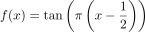 is continuous because it is a composition of continuous functions. The restriction
  is bijective with continuous inverse
  . Therefore is bijective and its inverse
 is a homeomorphism.
Stereographic projection
The Euclidean plane  is homeomorphic to the 2-sphere minus one point, denoted
  where
where  is the north pole.
HTTP-Response:
Error 400: ! Text line contains an invalid character.
l.70 ...) node[anchor=south west, text=black] {^^?
(exit code 1)
Diagram-Code:
\documentclass[tikz,border=15pt]{standalone}
\usepackage{tikz-3dplot}
\usetikzlibrary{calc, arrows.meta}
\begin{document}
\def\viewTheta{70}
\def\viewPhi{20}
\tdplotsetmaincoords{\viewTheta}{\viewPhi}
\begin{tikzpicture}[tdplot_main_coords, scale=2, line cap=round, line join=round]
\def\R{1}
\coordinate (O) at (0,0,0);
\coordinate (N) at (0,0,\R);
\def\thetaS{60}
\def\phiS{30}
\pgfmathsetmacro{\px}{\R * sin(\thetaS) * cos(\phiS)}
\pgfmathsetmacro{\py}{\R * sin(\thetaS) * sin(\phiS)}
\pgfmathsetmacro{\pz}{\R * cos(\thetaS)}
\coordinate (P) at (\px, \py, \pz);
\pgfmathsetmacro{\ux}{\px / (1 - \pz)}
\pgfmathsetmacro{\uy}{\py / (1 - \pz)}
\coordinate (Pprime) at (\ux, \uy, 0);
\pgfmathsetmacro{\eqFrontStart}{\viewPhi - 180}
\pgfmathsetmacro{\eqFrontEnd}{\viewPhi}
\pgfmathsetmacro{\eqBackStart}{\viewPhi - 180}
\pgfmathsetmacro{\eqBackEnd}{\viewPhi+180}
\pgfmathsetmacro{\cotViewTheta}{cos(\viewTheta)/sin(\viewTheta)}
\pgfmathsetmacro{\cotThetaS}{cos(\thetaS)/sin(\thetaS)}
\pgfmathsetmacro{\cosAlpha}{max(min(-\cotThetaS * \cotViewTheta, 1), -1)}
\pgfmathsetmacro{\alpha}{acos(\cosAlpha)}
\pgfmathsetmacro{\latFrontStart}{\viewPhi-180}
\pgfmathsetmacro{\latFrontEnd}{\viewPhi}
\pgfmathsetmacro{\latBackStart}{\viewPhi}
\pgfmathsetmacro{\latBackEnd}{\viewPhi+180}
\draw[thick, black] (-1.2,0,0) -- (0,0,0);
\draw[thick, black] (0,-3,0) -- (0,0,0);
\draw[thick, black] (0,0,-1.2) -- (0,0,0);
\draw[thick, ->, >=Stealth] (0,0,0) -- (2.2,0,0) node[anchor=north east]{$x$};
\draw[thick, ->, >=Stealth] (0,0,0) -- (0,3.0,0) node[anchor=north west]{$y$};
\draw[thick, dashed] (0,0,0) -- (N);
\draw[thick, ->, >=Stealth] (N) -- (0,0,1.8) node[anchor=south]{$z$};
\begin{scope}[tdplot_screen_coords]
\shade[ball color=cyan, opacity=0.15] (0,0) circle (\R);
\draw[cyan!60!blue, thick] (0,0) circle (\R);
\end{scope}
\tdplotdrawarc[cyan!60!blue, thick]{(O)}{\R}{\eqFrontStart}{\eqFrontEnd}{}{}
\tdplotdrawarc[cyan!60!blue, thin, dashed]{(O)}{\R}{\eqBackStart}{\eqBackEnd}{}{}
\pgfmathsetmacro{\rLat}{\R * sin(\thetaS)}
\coordinate (CenterLat) at (0,0,\pz);
\tdplotsetrotatedcoords{0}{0}{0}
\tdplotsetrotatedcoordsorigin{(CenterLat)}
\tdplotdrawarc[cyan!70!black, thin, dashed, tdplot_rotated_coords]{(0,0,0)}{\rLat}{\latBackStart}{\latBackEnd}{}{}
\tdplotdrawarc[cyan!70!black, thin, tdplot_rotated_coords]{(0,0,0)}{\rLat}{\latFrontStart}{\latFrontEnd}{}{}
\tdplotsetrotatedcoordsorigin{(O)}
\draw[red, thick, dashed] (N) -- (P);
\draw[red, thick, ->, >=Stealth] (P) -- (Pprime);
\fill[black] (N) circle (0.8pt) node[anchor=south east] {$N$};
\fill[red] (P) circle (1pt) node[anchor=south west, text=black] { };
\fill[red] (Pprime) circle (1pt) node[anchor=north west, text=black] {
};
\fill[red] (Pprime) circle (1pt) node[anchor=north west, text=black] { };
\end{tikzpicture}
\end{document}
};
\end{tikzpicture}
\end{document}
Define the stereographic projection  by
by

 on
on  ).
).
The inverse map  is given by

 and
and  by direct substitution. Hence
  is a homeomorphism.
Quotient space
The unit interval  with the endpoints identified (the quotient space
  where
where  ) is homeomorphic to the circle
  .
.
Define the map  by
by

 .
.
Consider the equivalence relation  , and let
  be the quotient map. By the universal property of the quotient map, there exists a unique continuous map
  such that
  ; that is, the following diagram commutes.

The map  is bijective because:
- Surjectivity follows from surjectivity of ;
- Injectivity holds because
but in the latter case

 in the quotient.
Hence is a continuous bijection.
The space is compact as the quotient of a compact space, and is Hausdorff. By the Compact-to-Hausdorff theorem, a continuous bijection from a compact space to a Hausdorff space is a homeomorphism.
Therefore is a homeomorphism.
HTTP-Response:
Error 400: ! Text line contains an invalid character.
l.23 \node[label text] at (0,-2.6) {^^?
(exit code 1)
Diagram-Code:\documentclass[tikz,border=10pt]{standalone}
\usepackage{amsmath}
\usetikzlibrary{arrows.meta,calc}
\begin{document}
\begin{tikzpicture}[
>={Stealth[scale=1.1]},
dot/.style={circle,fill=black,inner sep=1.6pt},
label text/.style={font=\Large,align=center}
]
\def\r{1.4}
\def\gap{50}
\coordinate (C1) at (0,0);
\coordinate (C2) at (5.5,0);
\coordinate (C3) at (11,0);
\begin{scope}[shift={(C1)}]
\draw[thick] (-\r,0) coordinate (A) -- (\r,0) coordinate (B);
\node[dot] at (A) {};
\node[dot] at (B) {};
\node[label text] at (0,-2.6) {};
\coordinate (R1) at (\r,0);
\end{scope}
\draw[->,thick] ( ) -- (
 )
node[midway,above] {$q$};
\begin{scope}[shift={(C2)}]
\draw[thick]
(180-\gap:\r)
arc[start angle=180-\gap,end angle=360+\gap,radius=\r];
\node[dot] (L) at (180-\gap:\r) {};
\node[dot] (R) at (\gap:\r) {};
\draw[dashed,->,thick]
(L) .. controls +(0,0) and +(-0.8,-0.1) .. (90:\r);
\draw[dashed,->,thick]
(R) .. controls +(0,0) and +(0.8,-0.1) .. (90:\r);
\node[label text] at (0,-2.6)
{ \\[-0.4ex]\normalsize
)
node[midway,above] {$q$};
\begin{scope}[shift={(C2)}]
\draw[thick]
(180-\gap:\r)
arc[start angle=180-\gap,end angle=360+\gap,radius=\r];
\node[dot] (L) at (180-\gap:\r) {};
\node[dot] (R) at (\gap:\r) {};
\draw[dashed,->,thick]
(L) .. controls +(0,0) and +(-0.8,-0.1) .. (90:\r);
\draw[dashed,->,thick]
(R) .. controls +(0,0) and +(0.8,-0.1) .. (90:\r);
\node[label text] at (0,-2.6)
{ \\[-0.4ex]\normalsize  };
\coordinate (R2) at (2,0);
\end{scope}
\draw[->,thick] (
};
\coordinate (R2) at (2,0);
\end{scope}
\draw[->,thick] ( ) -- (
 )
node[midway,above] {
)
node[midway,above] { };
\begin{scope}[shift={(C3)}]
\draw[thick] (0,0) circle (\r);
\node[dot] at (90:\r) {};
\node[label text] at (0,-2.6) {
};
\begin{scope}[shift={(C3)}]
\draw[thick] (0,0) circle (\r);
\node[dot] at (90:\r) {};
\node[label text] at (0,-2.6) { };
\end{scope}
\end{tikzpicture}
\end{document}
};
\end{scope}
\end{tikzpicture}
\end{document}Counterexamples
is not homeomorphic to .
For contradiction, suppose that there exists a homeomorphism  .
.
Consider the subspace  of . The restriction on it,
  is also a homeomorphism.
However, has two connected components,  and
and  , while
  is connected, which contradicts the assumption that the two spaces are homeomorphic.
HTTP-Response:
Error 400: ! Text line contains an invalid character.
l.20 \node[font=\Large] at (0, -2) {^^?
(exit code 1)
Diagram-Code:
\documentclass[tikz, border=10pt]{standalone}
\usepackage{amsmath, amssymb}
\begin{document}
\begin{tikzpicture}
\begin{scope}[xshift=-5cm]
\draw[thick] (-3, 0) -- (3, 0);
\filldraw[fill=white, draw=black, thick] (0, 0) circle (2.5pt);
\draw[cyan!60!blue, very thick] (-2.5, 0) -- (-1, 0);
\fill[cyan!60!blue] (-2.5, 0) circle (2pt);
\fill[cyan!60!blue] (-1, 0) circle (2pt);
\draw[cyan!60!blue, very thick] (1.3, 0) -- (2.2, 0);
\fill[cyan!60!blue] (1.3, 0) circle (2pt);
\fill[cyan!60!blue] (2.2, 0) circle (2pt);
\node[font=\Large] at (0, -2) { };
\end{scope}
\begin{scope}[xshift=4cm]
\draw[thick] (-3.5, -2.5) -- (3.5, -2.5) -- (3.5, 2.5) -- (-3.5, 2.5) -- cycle;
\filldraw[fill=white, draw=black, thick] (-0.3, -0.2) circle (2.5pt);
\draw[cyan!60!blue, very thick] (-2, 1.5) .. controls (-0.5, 1) and (-0.8, -1) .. (-1.2, -1.8);
\fill[cyan!60!blue] (-2, 1.5) circle (2pt);
\fill[cyan!60!blue] (-1.2, -1.8) circle (2pt);
\draw[cyan!60!blue, very thick] (-0.3, 1.5) .. controls (1.5, 1.8) and (2.5, 1) .. (2, 0.5);
\fill[cyan!60!blue] (-0.3, 1.5) circle (2pt);
\fill[cyan!60!blue] (2, 0.5) circle (2pt);
\draw[cyan!60!blue, very thick] (-0.3, 0.5) .. controls (1, 0) and (1, -1) .. (2.5, -2);
\fill[cyan!60!blue] (-0.3, 0.5) circle (2pt);
\fill[cyan!60!blue] (2.5, -2) circle (2pt);
\draw[cyan!60!blue, very thick] (-0.5, -0.8) .. controls (0, -1.8) and (1, -1.5) .. (0.8, -1);
\fill[cyan!60!blue] (-0.5, -0.8) circle (2pt);
\fill[cyan!60!blue] (0.8, -1) circle (2pt);
\node[font=\Large] at (0, -3.5) {
};
\end{scope}
\begin{scope}[xshift=4cm]
\draw[thick] (-3.5, -2.5) -- (3.5, -2.5) -- (3.5, 2.5) -- (-3.5, 2.5) -- cycle;
\filldraw[fill=white, draw=black, thick] (-0.3, -0.2) circle (2.5pt);
\draw[cyan!60!blue, very thick] (-2, 1.5) .. controls (-0.5, 1) and (-0.8, -1) .. (-1.2, -1.8);
\fill[cyan!60!blue] (-2, 1.5) circle (2pt);
\fill[cyan!60!blue] (-1.2, -1.8) circle (2pt);
\draw[cyan!60!blue, very thick] (-0.3, 1.5) .. controls (1.5, 1.8) and (2.5, 1) .. (2, 0.5);
\fill[cyan!60!blue] (-0.3, 1.5) circle (2pt);
\fill[cyan!60!blue] (2, 0.5) circle (2pt);
\draw[cyan!60!blue, very thick] (-0.3, 0.5) .. controls (1, 0) and (1, -1) .. (2.5, -2);
\fill[cyan!60!blue] (-0.3, 0.5) circle (2pt);
\fill[cyan!60!blue] (2.5, -2) circle (2pt);
\draw[cyan!60!blue, very thick] (-0.5, -0.8) .. controls (0, -1.8) and (1, -1.5) .. (0.8, -1);
\fill[cyan!60!blue] (-0.5, -0.8) circle (2pt);
\fill[cyan!60!blue] (0.8, -1) circle (2pt);
\node[font=\Large] at (0, -3.5) { };
\end{scope}
\end{tikzpicture}
\end{document}
};
\end{scope}
\end{tikzpicture}
\end{document}
Hence, no such homeomorphism exists; therefore is not homeomorphic to
The map from the interval  to the 1-sphere ,

is continuous and bijective, but not a homeomorphism.
HTTP-Response:
Error 400: ! Text line contains an invalid character.
l.15 ...1.2) to[bend left=30] node[above=2pt] {^^?
(exit code 1)
Diagram-Code:
\documentclass{article}
\usepackage{tikz}
\usetikzlibrary{arrows.meta}
\begin{document}
\begin{tikzpicture}
\draw (0,0) -- (4,0);
\draw (0.15, 0.25) -- (0, 0.25) -- (0, -0.25) -- (0.15, -0.25);
\draw (3.9, 0.25) to[bend left=45] (3.9, -0.25);
\draw[-{Stealth[length=3mm, width=2mm]}] (4.5, 1.2) to[bend left=30] node[above=2pt] { } (7.0, 1.2);
\draw (9.5, 0) circle (2);
\begin{scope}[rotate around={90:(11.5,0)}]
\draw (11.39, 0.25) to[bend left=45] (11.39, -0.25);
\draw (11.5, -0.25) -- (11.5, 0.25);
\draw (11.5, 0.25) -- (11.65, 0.25);
\draw (11.5, -0.25) -- (11.65, -0.25);
\end{scope}
\end{tikzpicture}
\end{document}
} (7.0, 1.2);
\draw (9.5, 0) circle (2);
\begin{scope}[rotate around={90:(11.5,0)}]
\draw (11.39, 0.25) to[bend left=45] (11.39, -0.25);
\draw (11.5, -0.25) -- (11.5, 0.25);
\draw (11.5, 0.25) -- (11.65, 0.25);
\draw (11.5, -0.25) -- (11.65, -0.25);
\end{scope}
\end{tikzpicture}
\end{document}
The map is:
- Continuous, as it is the composition of continuous maps
 and
and  .
. - Injective, because if
 , then
  . Since
  , it follows that
  .
. - Surjective, since every point of can be written as
 for some
  .
.
Hence is a continuous bijection.
However, is not a homeomorphism.
Consider the sequence

 in . But

 in . Thus
  is not continuous.
Topological invariants
A topological invariant is a property of a topological space that is preserved under homeomorphisms. In other words, if two spaces are homeomorphic, they either both possess the property or both do not. Invariants are the important tools to classify topological spaces. If two spaces differ in any topological invariant, they cannot be homeomorphic. Conversely, showing that two spaces share many invariants is often the first step on proving they are homeomorpic, though it is never sufficient by itself.
Common topological invariants
- Connectedness
- Compactness
- Hausdorff property
- Cardinality of the space
Algebraic invariants
More powerful invariants come from algebraic topology, which assigns algebraic objects to topological spaces.
Homeomorphism group
The collection of all autohomeomorphisms of a topological space forms a group under composition operation, known as the homeomorphism group of , denoted  . The homeomorphism group captures the symmetry in topology. It describes the ways in which a topological space can be continuously transformed onto itself.
The homeomorphism group is a faithful group action on its underlying set . It moves points in continuously onto itself, and the topological structure of is also reflected in the algebraic invariants such as the orbits and stabilizers of the action.
For example, consider the 2-sphere  as a thin rubber membrane tightly wraped around a ball. Each autohomeomorphism of , which is an element in
  , corresponds to a continuous deformation of this membrane. This operation can be stretching, bending, twisting, or any composition of these operations, so the rubber always remains attached to the ball.
HTTP-Response:
Error 400: ! Text line contains an invalid character.
l.39 node[midway, above, font=\small] {^^?
(exit code 1)
Diagram-Code:
\documentclass[tikz,border=5mm]{standalone}
\usetikzlibrary{arrows.meta, positioning, calc}
\usepackage{amssymb}
\begin{document}
\begin{tikzpicture}[scale=1.2, >=Stealth]
\begin{scope}[shift={(0,0)}]
\shade[ball color=cyan, opacity=0.2] (0,0) circle (2);
\draw[cyan!60!blue, thick] (-2,0) arc (180:360:2 and 0.25);
\draw[cyan!60!blue, thin, dashed] (2,0) arc (0:180:2 and 0.25);
\foreach \y in {-1.2, -0.6, 0.6, 1.2} {
\pgfmathsetmacro{\x}{sqrt(4-\y*\y)}
\draw[cyan!70!black, thin] (-\x, \y) arc (180:360:\x cm and 0.25cm);
\draw[cyan!70!black, thin, dashed] (\x, \y) arc (0:180:\x cm and 0.25cm);
}
\draw[cyan!70!black, thin] (0,2) arc (90:-90:0.6 and 2);
\draw[cyan!70!black, thin] (0,2) arc (90:-90:1.3 and 2);
\draw[cyan!70!black, thin] (0,2) arc (90:270:0.6 and 2);
\draw[cyan!70!black, thin] (0,2) arc (90:270:1.3 and 2);
\draw[cyan!70!black, thin] (0,2) -- (0,-2);
\filldraw[fill=yellow!60, draw=yellow!60!black, thick, opacity=0.7]
(0.7, 1.1) .. controls (1.0, 1.3) and (1.3, 1.1) .. (1.4, 0.5)
.. controls (1.1, 0.1) and (0.1, 0.6) .. (0.7, 1.1)
-- cycle;
\node[yellow!60!black, font=\bfseries] at (1.1, 0.9) {$U$};
\filldraw[black] (0.8, 0.9) circle (1pt) node[anchor=south east, scale=0.8] {$x$};
\filldraw[black] (1.1, 0.7) circle (1pt) node[anchor=north west, scale=0.8] {$y$};
\node[below, text=black] at (0,-2.3) {$X$};
\draw[cyan!60!blue, thick] (0,0) circle (2);
\end{scope}
\draw[->, thick, black] (2.5, 0) -- (4.5, 0)
node[midway, above, font=\small] { };
\begin{scope}[shift={(7,0)}]
\shade[ball color=cyan, opacity=0.2] (0,0) circle (2);
\draw[cyan!60!blue, thick] (-2.0,0.0) .. controls (-0.9, -0.3) and (0.9, 0.3) .. (2.0, 0.0);
\draw[cyan!60!blue, thin, dashed] (2.0,0.0) .. controls (0.9, 0.6) and (-0.9, 0.0) .. (-2.0, 0.0);
\draw[cyan!70!black, thin] (-1.6, 1.2) .. controls (-0.6, 0.9) and (0.6, 1.5) .. (1.6, 1.2);
\draw[cyan!70!black, thin, dashed] (1.6, 1.2) .. controls (0.6, 1.6) and (-0.6, 1.0) .. (-1.6, 1.2);
\draw[cyan!70!black, thin] (-1.9, 0.6) .. controls (-0.9, 0.3) and (0.9, 0.9) .. (1.9, 0.6);
\draw[cyan!70!black, thin, dashed] (1.9, 0.6) .. controls (0.9, 1.1) and (-0.9, 0.5) .. (-1.9, 0.6);
\draw[cyan!70!black, thin] (-1.9, -0.6) .. controls (-0.9, -0.9) and (0.9, -0.3) .. (1.9, -0.6);
\draw[cyan!70!black, thin, dashed] (1.9, -0.6) .. controls (0.9, -0.1) and (-0.9, -0.5) .. (-1.9, -0.6);
\draw[cyan!70!black, thin] (-1.6, -1.2) .. controls (-0.6, -1.5) and (0.6, -0.9) .. (1.6, -1.2);
\draw[cyan!70!black, thin, dashed] (1.6, -1.2) .. controls (0.6, -0.8) and (-0.6, -1.4) .. (-1.6, -1.2);
\draw[cyan!70!black, thin] (0, 2) .. controls (-1.9, 0.8) and (-1.7, -1.2) .. (0, -2);
\draw[cyan!70!black, thin] (0, 2) .. controls (-1.1, 0.8) and (-0.9, -1.2) .. (0, -2);
\draw[cyan!70!black, thin] (0, 2) .. controls (-0.3, 0.8) and (-0.1, -1.2) .. (0, -2);
\draw[cyan!70!black, thin] (0, 2) .. controls (0.5, 0.8) and (0.7, -1.2) .. (0, -2);
\draw[cyan!70!black, thin] (0, 2) .. controls (1.3, 0.8) and (1.5, -1.2) .. (0, -2);
\draw[cyan!70!black, thin, dashed] (0, 2) .. controls (-1.3, 0.8) and (-0.8, -1.2) .. (0, -2);
\draw[cyan!70!black, thin, dashed] (0, 2) .. controls (0.9, 0.8) and (0.5, -1.2) .. (0, -2);
\filldraw[fill=yellow!60, draw=yellow!60!black, thick, opacity=0.7]
(0.05, 1.3)
.. controls (0.4, 1.4) and (0.9, 1.5) .. (1.2, 0.7)
.. controls (0.9, 0.3) and (0.4, 0.15) .. (0.05, 0.5)
.. controls (-0.1, 0.8) and (-0.1, 1.1) .. (0.05, 1.3)
-- cycle;
\node[yellow!60!black, font=\bfseries] at (0.6, 0.95) {
};
\begin{scope}[shift={(7,0)}]
\shade[ball color=cyan, opacity=0.2] (0,0) circle (2);
\draw[cyan!60!blue, thick] (-2.0,0.0) .. controls (-0.9, -0.3) and (0.9, 0.3) .. (2.0, 0.0);
\draw[cyan!60!blue, thin, dashed] (2.0,0.0) .. controls (0.9, 0.6) and (-0.9, 0.0) .. (-2.0, 0.0);
\draw[cyan!70!black, thin] (-1.6, 1.2) .. controls (-0.6, 0.9) and (0.6, 1.5) .. (1.6, 1.2);
\draw[cyan!70!black, thin, dashed] (1.6, 1.2) .. controls (0.6, 1.6) and (-0.6, 1.0) .. (-1.6, 1.2);
\draw[cyan!70!black, thin] (-1.9, 0.6) .. controls (-0.9, 0.3) and (0.9, 0.9) .. (1.9, 0.6);
\draw[cyan!70!black, thin, dashed] (1.9, 0.6) .. controls (0.9, 1.1) and (-0.9, 0.5) .. (-1.9, 0.6);
\draw[cyan!70!black, thin] (-1.9, -0.6) .. controls (-0.9, -0.9) and (0.9, -0.3) .. (1.9, -0.6);
\draw[cyan!70!black, thin, dashed] (1.9, -0.6) .. controls (0.9, -0.1) and (-0.9, -0.5) .. (-1.9, -0.6);
\draw[cyan!70!black, thin] (-1.6, -1.2) .. controls (-0.6, -1.5) and (0.6, -0.9) .. (1.6, -1.2);
\draw[cyan!70!black, thin, dashed] (1.6, -1.2) .. controls (0.6, -0.8) and (-0.6, -1.4) .. (-1.6, -1.2);
\draw[cyan!70!black, thin] (0, 2) .. controls (-1.9, 0.8) and (-1.7, -1.2) .. (0, -2);
\draw[cyan!70!black, thin] (0, 2) .. controls (-1.1, 0.8) and (-0.9, -1.2) .. (0, -2);
\draw[cyan!70!black, thin] (0, 2) .. controls (-0.3, 0.8) and (-0.1, -1.2) .. (0, -2);
\draw[cyan!70!black, thin] (0, 2) .. controls (0.5, 0.8) and (0.7, -1.2) .. (0, -2);
\draw[cyan!70!black, thin] (0, 2) .. controls (1.3, 0.8) and (1.5, -1.2) .. (0, -2);
\draw[cyan!70!black, thin, dashed] (0, 2) .. controls (-1.3, 0.8) and (-0.8, -1.2) .. (0, -2);
\draw[cyan!70!black, thin, dashed] (0, 2) .. controls (0.9, 0.8) and (0.5, -1.2) .. (0, -2);
\filldraw[fill=yellow!60, draw=yellow!60!black, thick, opacity=0.7]
(0.05, 1.3)
.. controls (0.4, 1.4) and (0.9, 1.5) .. (1.2, 0.7)
.. controls (0.9, 0.3) and (0.4, 0.15) .. (0.05, 0.5)
.. controls (-0.1, 0.8) and (-0.1, 1.1) .. (0.05, 1.3)
-- cycle;
\node[yellow!60!black, font=\bfseries] at (0.6, 0.95) { };
\filldraw[black] (0.4, 1.1) circle (1pt) node[anchor=south east, scale=0.8] {
};
\filldraw[black] (0.4, 1.1) circle (1pt) node[anchor=south east, scale=0.8] { };
\filldraw[black] (0.8, 0.6) circle (1pt) node[anchor=north west, scale=0.8] {
};
\filldraw[black] (0.8, 0.6) circle (1pt) node[anchor=north west, scale=0.8] { };
\node[below, text=black] at (0,-2.3) {
};
\node[below, text=black] at (0,-2.3) { };
\draw[cyan!60!blue, thick] (0,0) circle (2);
\end{scope}
\end{tikzpicture}
\end{document}
};
\draw[cyan!60!blue, thick] (0,0) circle (2);
\end{scope}
\end{tikzpicture}
\end{document}
Under the natural action of , every point on the sphere can be moved continuously to any other point. This example shows how the homeomorphism group captures the symmetry of a topological space in the perspective of continuity.